هشدارها درباره نزدیک شدن به سررسید در اکسل

Question

جاناتان یک کاربرگ ایجاد کرد که تاریخ سررسید اسناد مختلف بخش را ردیابی می کند. او فکر کرد که آیا راهی برای اکسل وجود دارد که به نحوی به او هشدار دهد که آیا موعد مقرر برای یک سند خاص نزدیک است.

روش های مختلفی برای انجام این کار در اکسل وجود دارد و شما باید بهترین روش را برای اهداف خود انتخاب کنید. روش اول این است که به سادگی یک ستون به کاربرگ خود اضافه کنید که برای هشدار استفاده می شود. با فرض اینکه تاریخ سررسید شما در ستون F باشد، می توانید فرمول زیر را در ستون G قرار دهید:

=IF(F3

The formula checks to see if the date in cell F3 is earlier than a week from today. If so, then the formula displays "<</p>

Another approach is to use the conditional formatting capabilities of Excel. Follow these steps:

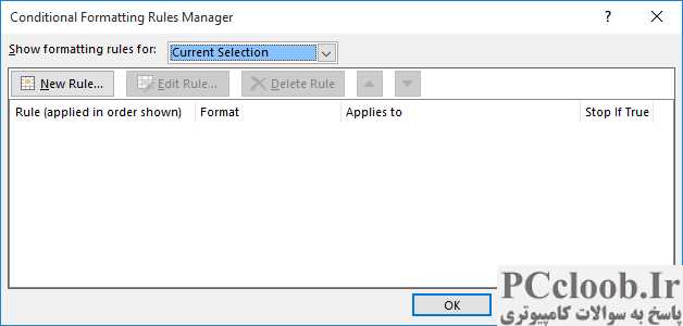
Figure 1. The Conditional Formatting Rules Manager dialog box.

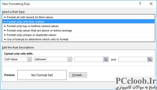
Figure 2. The New Formatting Rule dialog box.

1. Select the cells that contain the document due dates.
2. Make sure the Home tab of the ribbon is displayed.
3. Click the Conditional Formatting option in the Styles group. On the resulting submenu, click Manage Rules. Excel displays the Conditional Formatting Rules Manager dialog box. (See Figure 1.)
4. Click the New Rule button. Excel displays the New Formatting Rule dialog box.
5. In the Select a Rule Type list, choose Format Only Cells That Contain. (See Figure 2.)
6. Make sure the first drop-down list in the Edit the Rule Description area is "Cell Value." (This should be the default.)
7. Make sure the second drop-down list is "Less Than."
8. In the formula area, enter "=TODAY()" (without the quote marks).
9. Click the Format button. Excel displays the Format Cells dialog box.
10. Using the Color drop-down list, choose the color red.
11. Click OK to close the Format Cells dialog box.
12. Click OK. The Conditional Formatting Rules Manager dialog box reappears with your newly defined condition in it.
13. Click the New Rule button. Excel displays the New Formatting Rule dialog box.
14. In the Select a Rule Type List, choose Format Only Cells That Contain.
15. Make sure the first drop-down list in the Edit the Rule Description area is "Cell Value." (This should be the default.)
16. Make sure the second drop-down list is "Less Than."
17. In the formula area, enter "=TODAY()+7" (without the quote marks).
18. Click the Format button. Excel displays the Format Cells dialog box.
19. Using the Color drop-down list, choose the color blue.
20. Click OK to close the Format Cells dialog box.
21. Click OK. The Conditional Formatting Rules Manager dialog box reappears with your newly defined condition in it. (The newly defined condition should actually be selected in the list of conditions.)
22. Click the Move Down arrow. This moves the last condition you defined (steps 13 through 21) so it is in the proper order.
23. Click OK to close the Conditional Formatting dialog box.

This is a two-tiered format, and you end up with two levels of alert. If the due date is already past, then it shows up as red. If the due date is today or within the next seven days, then it shows up in blue.